Setting up the case studies: Atlantic and Gulf of Thailand
Source:vignettes/scenario-setup.Rmd
scenario-setup.RmdThis vignette documents how the two example systems of the package
were built and tuned, as a guideline for setting up your own: the input
tables, how catchability was derived, the fleet settings that shape
behaviour, and the calibration of the starting point. Part A covers the
Atlantic example (atlantic_system()), Part B the Gulf of
Thailand draft (got_system_draft()), and Part C summarises
the steps as a checklist. The model itself is described in
vignette("how-it-works"), and the analysis functions in
vignette("mmsyFM").
library(mmsyFM)
library(ggplot2)
ext <- function(f) read.csv(system.file("extdata", f, package = "mmsyFM"), check.names = FALSE)
Part A: the Atlantic example
A generic north-east Atlantic mixed hook-and-line fishery with ten stocks: six demersal (from reef fish to hake) and four pelagic (two of them seasonal migrants). It is a conceptual system for exploring mixed-fishery management, not an assessment of real stocks.
A1. Stocks
ext("atlantic_species.csv")
#>                  species code    group    r    K price season_amp season_peak
#> 1          Dentex dentex  DEC demersal 0.25  500    12        0.0           1
#> 2    Pagellus erythrinus  PAC demersal 0.35  900     8        0.0           1
#> 3     Pagellus bogaraveo  SBR demersal 0.18  800    15        0.0           1
#> 4  Merluccius merluccius  HKE demersal 0.30 2500     5        0.0           1
#> 5          Conger conger  COE demersal 0.30  600     3        0.0           1
#> 6      Phycis blennoides  GFB demersal 0.30  700     2        0.0           1
#> 7       Thunnus alalunga  ALB  pelagic 0.40 3000     6        0.7           9
#> 8    Coryphaena hippurus  DOL  pelagic 0.80 1500     7        0.9           9
#> 9       Seriola dumerili  AMB  pelagic 0.35  600     9        0.4           8
#> 10        Scomber colias  VMA  pelagic 0.80 4000     2        0.3           5
Growth rates (r), carrying capacities (K)
and relative prices are indicative. Pelagic stocks have seasonal
availability (season_amp, peak month
season_peak), so their catch rates vary through the
year.
A2. Metiers and catchability: from a habitat landscape
The metiers are three tactics (reef handline, sediment longline, pelagic troll) on two grounds (shallow and deep, split at 300 m), i.e. six metiers. Their catchability was derived once from the spatial multispecies simulator of the cpueTargeting package, which re-implements the simulator of Thorson et al. (2017), itself generalising Ono et al. (2015):
- a habitat landscape of depth, reef patches and sea-surface temperature on a grid; each species has a depth, substrate (reef or sediment) and, for pelagics, temperature preference, giving its spatial distribution at K;
- each metier fishes the cells of its ground (shallow or deep, reef or sediment, or the water column for the troll) with a gear selectivity for each species;
- catchability = selectivity x the mean share of the stock’s K per cell of the ground, with fishing spread evenly over the ground.
Two settings were changed from the logbook simulator to give a
balanced system: the selectivity of the pelagic troll for Seriola
dumerili was lowered from 0.8 to 0.4 (with 0.8, the reef and troll
by-catch drove it down under open access), and mixed vessels fish at
0.75 of the specialists’ efficiency. The resulting matrix is stored as a
table, so the package does not depend on cpueTargeting;
ms_landscape() (Part B) is the stand-alone equivalent of
this step.
sys_a <- atlantic_system()
plot_catchability(sys_a)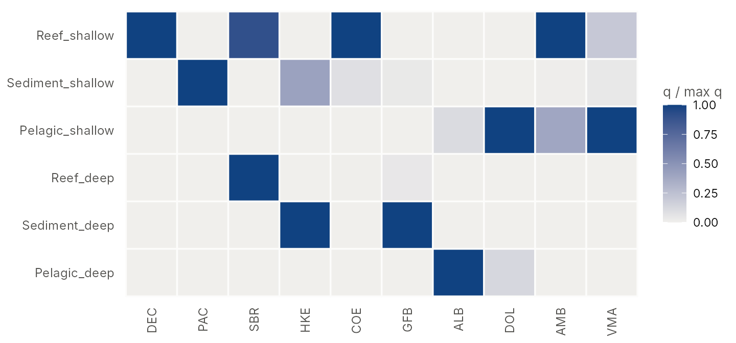
Dentex dentex lives on a narrow reef habitat and has the highest catchability relative to its growth rate: it becomes the choke stock.
A3. Fleet segments
ext("atlantic_segments.csv")
#>    segment share_target loyalty efficiency cost_multiplier vessel_cv
#> 1 demersal         0.35     0.8       1.00          0.6340      0.25
#> 2  pelagic         0.35     0.8       1.00          1.0774      0.25
#> 3    mixed         0.30     0.0       0.75          0.8434      0.25
#>                                                                                 home
#> 1                              Reef_shallow;Sediment_shallow;Reef_deep;Sediment_deep
#> 2                                                       Pelagic_shallow;Pelagic_deep
#> 3 Reef_shallow;Sediment_shallow;Pelagic_shallow;Reef_deep;Sediment_deep;Pelagic_deep- Demersal and pelagic specialists fish 80% of their days on their home metiers (loyalty 0.8) and the rest wherever it pays best.
- The mixed segment is a generalist (loyalty 0) at 0.75 efficiency.
- Each metier’s daily cost is 0.4 of its unfished revenue rate
(
costin the metier table); the segment multipliers (cost_multiplier) are tuned. -
vessel_cv = 0.25: vessel efficiency varies within a segment, so some vessels break even while others stay in port.
A4. Tuning the status quo
The daily cost multipliers were solved with ms_tune() so
that the open-access equilibrium (capacity 1,000 days per segment,
gamma = 1.5) has 35 / 35 / 30% of the days by segment and
the weakest stock at 0.4 Bmsy:
sys_a <- ms_tune(sys_a, shares = c(demersal = 0.35, pelagic = 0.35, mixed = 0.30),
                 status = c(min = 0.4), cap = 1000, gamma = 1.5)
The stored system is the result:
sq_a <- ms_status_quo(sys_a, capacity = 1000, gamma = 1.5, years = 300)
round(sq_a$E_seg / sum(sq_a$E_seg), 2)
#> demersal  pelagic    mixed
#>     0.36     0.34     0.30
round(sort(sq_a$BBmsy), 2)
#>         Dentex dentex      Seriola dumerili    Pagellus bogaraveo
#>                  0.40                  0.47                  0.50
#> Merluccius merluccius   Pagellus erythrinus     Phycis blennoides
#>                  0.51                  0.55                  0.70
#>      Thunnus alalunga         Conger conger   Coryphaena hippurus
#>                  0.73                  0.97                  1.05
#>        Scomber colias
#>                  1.14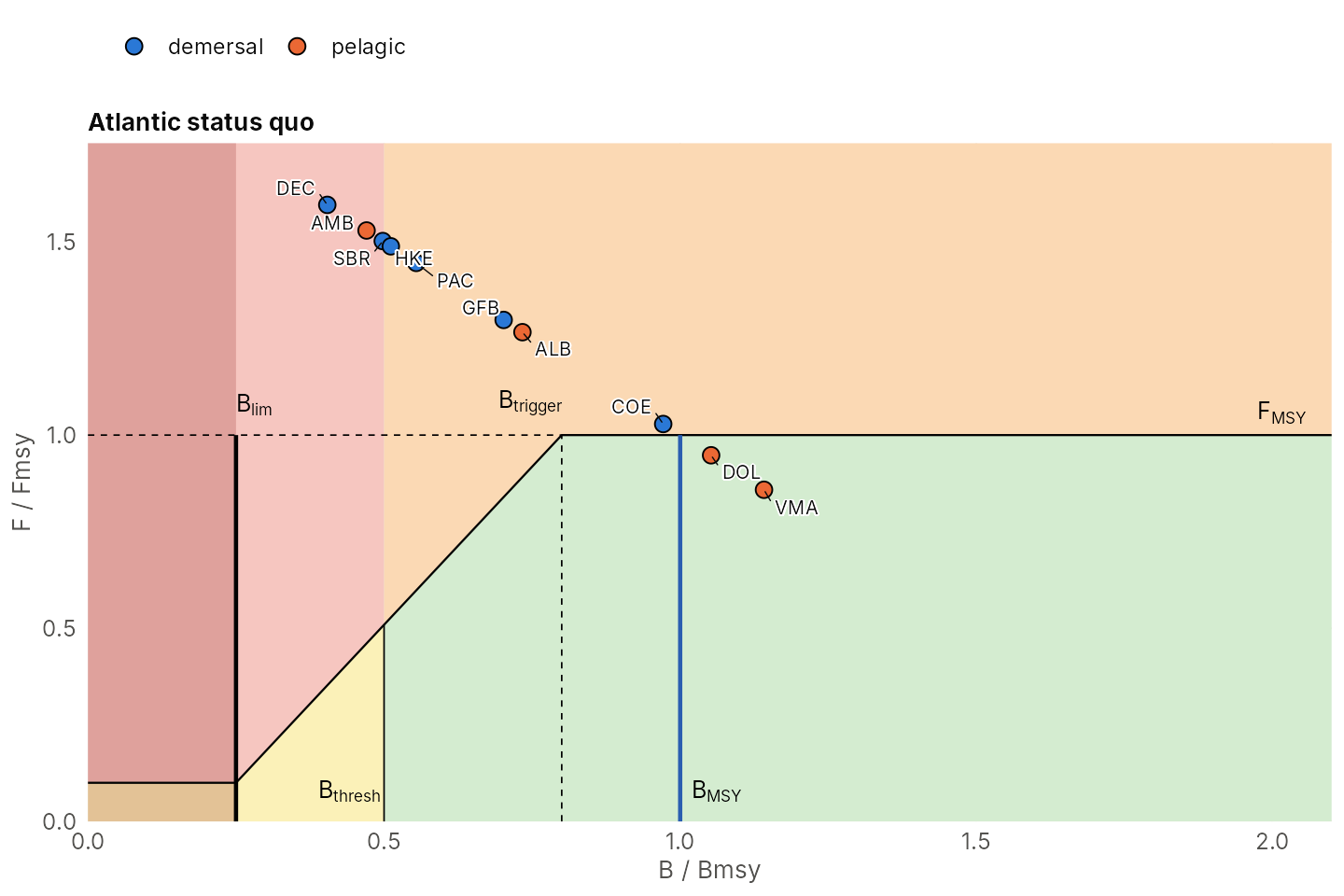
At the status quo Dentex, blackspot seabream and Seriola are the most depleted stocks (about 0.4-0.5 Bmsy), while the fast pelagics are above Bmsy.
Part B: the Gulf of Thailand draft
The Gulf of Thailand system represents the multispecies trawl, purse-seine and small-scale fisheries of the Gulf with the 18 species groups of the multispecies MSY app (mmsyapp), plus anchovies and sardines. It shows how a system is calibrated to the observed status of the stocks.
The Gulf of Thailand system is a draft. Prices, gear overlaps, habitat preferences and costs are indicative; the 2024 depletions are those of the multispecies MSY app (mmsyapp).
B1. The four tables
A system is built by ms_system() from four tables (or
read from CSV files with read_ms_system()).
Species
One row per stock: growth rate r, carrying capacity
K and a relative price; optionally
seasonality, the F cap and the starting depletion.
species <- ext("got_species.csv")
species[, c("species", "code", "group", "r", "K", "price", "F_cap", "dep_init", "dep_2024")]
#>                    species code      group          r         K price F_cap
#> 1                 Snappers  SNP   demersal 0.04950501 194126.69   6.0  1.95
#> 2                Catfishes  CAT   demersal 0.05017967 195614.21   2.0  1.95
#> 3                 Croakers  CRO   demersal 0.05036881 647838.12   1.5  1.95
#> 4                     Rays  RAY   demersal 0.06395467 232757.01   1.5  1.95
#> 5                   Sharks  SHK   demersal 0.05732474 132829.20   2.0  1.95
#> 6            Swimming crab  CRB    benthic 0.35931673 202741.16   8.0  1.95
#> 7             Lizardfishes  LIZ   demersal 0.38499380 109345.96   1.2  1.95
#> 8             Cuttlefishes  CUT cephalopod 0.52284449 149444.43   5.0  1.95
#> 9                 Groupers  GRO   demersal 0.18180063  61519.10  10.0  1.95
#> 10 Scads (horse mackerels)  SCD    pelagic 0.17354501 912968.71   1.5  1.95
#> 11        Threadfin breams  TBR   demersal 0.18419943 657875.95   2.0  1.95
#> 12           Black pomfret  POM    pelagic 0.21435880  36399.87   8.0  1.95
#> 13               Hairtails  HAI    pelagic 0.21439199  59185.71   3.0  1.95
#> 14                 Shrimps  SHR    benthic 1.43877344 548802.35  10.0  1.95
#> 15                 Bigeyes  BIG   demersal 0.23928674 249308.65   1.2  1.95
#> 16   Indo-Pacific mackerel  IMK    pelagic 0.32530656 237056.62   2.5  1.95
#> 17        Spanish mackerel  SMK    pelagic 0.40113973 553338.85   6.0  1.95
#> 18                  Squids  SQD cephalopod 0.65758769 262876.70   6.0  1.95
#> 19               Anchovies  ANC    anchovy 1.20000000 575000.00   1.0  1.95
#> 20                Sardines  SAR    pelagic 1.00000000 400000.00   0.8  1.95
#>    dep_init dep_2024
#> 1    0.1696    0.166
#> 2    0.1509    0.151
#> 3    0.0411    0.058
#> 4    0.1781    0.178
#> 5    0.2276    0.227
#> 6    0.2312    0.231
#> 7    0.3386    0.338
#> 8    0.1499    0.150
#> 9    0.2776    0.273
#> 10   0.1372    0.136
#> 11   0.0708    0.070
#> 12   0.2467    0.247
#> 13   0.2858    0.286
#> 14   0.7499    0.974
#> 15   0.0255    0.028
#> 16   0.0796    0.078
#> 17   0.3717    0.372
#> 18   0.2489    0.248
#> 19   0.3679       NA
#> 20 0.3829 NA-
randKare the 18 mmsyapp groups; anchovies and sardines were added. -
F_cap = 1.95(units of Fmsy) is the persistence floor: no stock settles below 0.05 Bmsy (vignette("how-it-works"), section 2). -
dep_2024is the mmsyapp 2024 depletion (B/K), the target of the calibration in section B4;dep_initis the starting depletion of simulations, written by that calibration.
Metiers and segments
ext("got_metiers.csv")[, c("metier", "tactic", "ground")]
#>                 metier                                         tactic   ground
#> 1             SSF_crab                          Crab gillnet and trap  coastal
#> 2           SSF_shrimp                     Shrimp trammel and gillnet  coastal
#> 3  SSF_pelagic_gillnet                   Encircling and drift gillnet  coastal
#> 4        SSF_hook_trap                       Hook and line, fish trap  coastal
#> 5       SSF_cephalopod                        Cephalopod trap and jig  coastal
#> 6             TR_inner               Trawl inner shelf (15-30 m, mud) offshore
#> 7               TR_mid                      Trawl mid shelf (30-50 m) offshore
#> 8             TR_outer              Trawl outer shelf (50-80 m, sand) offshore
#> 9          PS_mackerel                      Mackerel/scad purse seine offshore
#> 10          PS_anchovy Light-luring anchovy/small-pelagic purse seine offshore
segments <- ext("got_segments.csv")
segments
#>       segment share_target loyalty efficiency cost_multiplier vessel_cv
#> 1       trawl         0.12       1      1.000          0.1815      0.25
#> 2 purse_seine         0.06       1      1.000          0.2931      0.25
#> 3 small_scale         0.82       1      0.075          0.0265      0.25
#>                                                                   home capacity
#> 1                                             TR_inner;TR_mid;TR_outer      450
#> 2                                               PS_mackerel;PS_anchovy      225
#> 3 SSF_crab;SSF_shrimp;SSF_pelagic_gillnet;SSF_hook_trap;SSF_cephalopod     3000
Three segments with coastal zoning (loyalty 1: a segment fishes only its own metiers):
- trawl: inner (15-30 m, mud), mid (30-50 m) and outer shelf (50-80 m);
- purse seine: a mackerel/scad seine and a light-luring anchovy seine;
- small-scale fisheries (SSF): five coastal tactics. SSF is the generalist, switching between tactics by profit, with a low efficiency (0.075 of an industrial vessel-day) and a matching low daily cost, and it fishes 82% of the days.
capacity is the registered days of each segment;
share_target the share of days the calibration aims at.
B2. Catchability
The catchability matrix (metiers x stocks) says which metiers catch which stocks and how strongly. There are two ways to build it.
Route A: an expert overlap matrix
Score each metier-stock pair as main fishery (1), by-catch (0.2) or none (0), and scale by r (so a day has a similar F/Fmsy effect on every stock). This is how the draft was started; the stored matrix is that start after calibration (section B4):
sys <- got_system_draft()
plot_catchability(sys)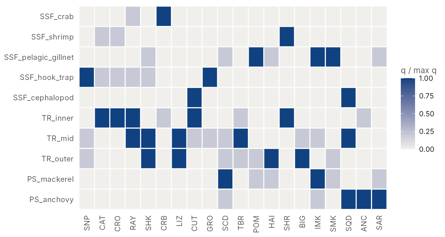
Route B: a habitat landscape
ms_landscape() derives catchability from where stocks
live and where and how metiers fish:
- seabed cells with depth, substrate and area;
- habitat preferences of each stock: a depth preference (mean, SD) and substrate weights;
- grounds of each metier: a depth range and substrates;
- gear selectivity of each metier for each stock.
cells <- ext("got_cells.csv")
habitat <- ext("got_habitat.csv")
grounds <- ext("got_grounds.csv")
sel <- ext("got_selectivity.csv")
head(habitat)
#>         species depth_mean depth_sd mud sand hard
#> 1      Snappers         40       12 0.2  0.6  1.0
#> 2     Catfishes         18        8 1.0  0.4  0.1
#> 3      Croakers         18        8 1.0  0.4  0.1
#> 4          Rays         35       12 1.0  0.8  0.2
#> 5        Sharks         55       12 0.4  1.0  0.4
#> 6 Swimming crab         12        7 1.0  0.8  0.2
grounds
#>                 metier depth_min depth_max substrate
#> 1             SSF_crab         0        15  mud;sand
#> 2           SSF_shrimp         0        15  mud;sand
#> 3  SSF_pelagic_gillnet         0        15
#> 4        SSF_hook_trap         0        15 hard;sand
#> 5       SSF_cephalopod         0        15
#> 6             TR_inner        15        30  mud;sand
#> 7               TR_mid        30        50  mud;sand
#> 8             TR_outer        50        80  mud;sand
#> 9          PS_mackerel        20        80
#> 10          PS_anchovy         5        40
The catchability is q0 x selectivity x the stock’s
density on the ground relative to its average density:
Q_land <- ms_landscape(cells, habitat, grounds, sel)
plot_landscape(Q_land, cells)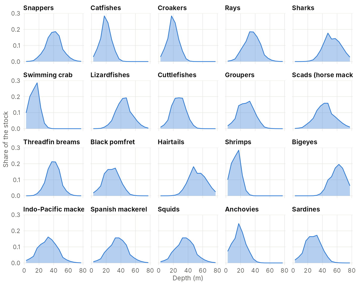
Each stock’s distribution over depth. Comparing the shape of each stock’s column (relative to its maximum) with the expert matrix:
nrm <- function(m) { m <- unclass(m); attributes(m) <- attributes(m)[c("dim", "dimnames")]
                     sweep(m, 2, apply(m, 2, max), "/") }
L <- nrm(Q_land); E <- nrm(sys$Q[rownames(L), ])
round(cor(as.vector(L), as.vector(E)), 2)
#> [1] 0.76
The landscape route is easier to defend and to change (e.g. a stock that moves deeper, a trawl ban inside 15 m), and it spreads catchability smoothly across grounds where the expert matrix has only 1, 0.2 and 0. Either way, the level of each stock’s catchability column is set by the calibration to the stock’s status; the matrix provides its shape.
To build a system from the landscape, pass it as the catchability:
sys_land <- ms_system(species, ext("got_metiers.csv")[, c("metier", "tactic", "ground")],
                      Q_land, segments)
sys_land
#> <ms_system> 20 stocks, 10 metiers, 3 segments
#>   stocks:   SNP, CAT, CRO, RAY, SHK, CRB, LIZ, CUT, GRO, SCD, TBR, POM, HAI, SHR, BIG, IMK, SMK, SQD, ANC, SAR
#>   metiers:  SSF_crab, SSF_shrimp, SSF_pelagic_gillnet, SSF_hook_trap, SSF_cephalopod, TR_inner, TR_mid, TR_outer, PS_mackerel, PS_anchovy
#>   segment trawl      loyalty 1.00, efficiency 1.00, daily cost x0.181, home: TR_inner, TR_mid, TR_outer
#>   segment purse_seine loyalty 1.00, efficiency 1.00, daily cost x0.293, home: PS_mackerel, PS_anchovy
#>   segment small_scale loyalty 1.00, efficiency 0.07, daily cost x0.026, home: SSF_crab, SSF_shrimp, SSF_pelagic_gillnet, SSF_hook_trap, SSF_cephalopod
#>   F cap:     1.95 x Fmsy
(Without a cost column, each metier’s daily cost is 0.4
of its unfished revenue rate.)
B3. Fleet behaviour
Two settings shape how the fleet responds:
-
Profit preference
gamma(“how strongly fishers chase profit”): each segment spreads its days over its metiers in proportion to expected profit per day raised togamma. 0 = profit-blind; 1.5 = a metier paying twice the profit gets 74% of the days. - Capacity: the registered days; the days actually fished are those of the vessels that break even.
The effect of gamma on where the days go at the status
quo:
cap <- c(trawl = 450, purse_seine = 225, small_scale = 3000)
days_by_metier <- function(g) {
  x <- ms_simulate(sys, matrix(cap, 1), 200, capacity = matrix(cap, 1), gamma = g, avg_years = 20)
  round(colMeans(x$E_metier[, 1, ]))
}
d <- sapply(c(0, 1.5, 3), days_by_metier)
dimnames(d) <- list(sys$metiers$name, paste("gamma", c(0, 1.5, 3)))
d
#>                     gamma 0 gamma 1.5 gamma 3
#> SSF_crab                597       104      16
#> SSF_shrimp              597      1659    1774
#> SSF_pelagic_gillnet     597      1038    1043
#> SSF_hook_trap           597       159     159
#> SSF_cephalopod          597        41       8
#> TR_inner                150       361     384
#> TR_mid                  150        54      41
#> TR_outer                150        35      25
#> PS_mackerel              99        95      95
#> PS_anchovy               99       124     127
With gamma = 0 every metier of a segment gets the same
days; with a strong preference, small-scale effort concentrates on the
shrimp and pelagic gillnet tactics, and trawl on the inner shelf.
B4. Calibrating the starting point
The calibration fixes what is not directly known (daily costs, the
level of each stock’s catchability) so that the open-access equilibrium
reproduces what is known: the fleet composition and the status of the
stocks. It runs once per scenario; the steps take 1-2 minutes each, so
they are shown here without running, and the results are those stored in
got_system_draft().
Step 1: daily costs. ms_tune() solves
each segment’s daily cost multiplier so that the open-access equilibrium
has the target shares of days (12 / 6 / 82%) and a target status (here:
the weakest stock at the 0.05 Bmsy floor):
Step 2: stock status. ms_condition()
rescales each stock’s catchability until its B/Bmsy matches the 2024
depletion (limited to 0.05-1.5 Bmsy; anchovies and sardines have no
value and are left free), keeping the shares of days with the total days
fixed:
target <- setNames(2 * species$dep_2024, species$species)   # B/Bmsy = 2 B/K
target <- target[!is.na(target)]
sys2 <- ms_condition(sys1, target, cap = cap, gamma = 1.5)
attr(sys2, "conditioning")            # targets, achieved B/Bmsy and F/Fmsy, q multipliers
Step 3: save the tables
(write_ms_system(sys2, "my_folder", "got")), so the
scenario can be reloaded with read_ms_system() or uploaded
in the app.
Checking the result
The stored draft went through these steps (from the expert matrix). Its status quo against the 2024 targets:
sq <- ms_status_quo(sys, capacity = cap, gamma = 1.5, years = 300)
round(sq$E_seg / sum(sq$E_seg), 3)                       # shares of days
#>       trawl purse_seine small_scale
#>       0.123       0.060       0.818
chk <- data.frame(stock = sys$code, target = pmin(pmax(2 * species$dep_2024, 0.05), 1.5),
                  BBmsy = round(sq$BBmsy, 2), FFmsy = round(sq$FFmsy, 2))
chk
#>                         stock target BBmsy FFmsy
#> Snappers                  SNP  0.332  0.34  1.66
#> Catfishes                 CAT  0.302  0.30  1.70
#> Croakers                  CRO  0.116  0.07  1.95
#> Rays                      RAY  0.356  0.36  1.64
#> Sharks                    SHK  0.454  0.46  1.54
#> Swimming crab             CRB  0.462  0.46  1.54
#> Lizardfishes              LIZ  0.676  0.68  1.32
#> Cuttlefishes              CUT  0.300  0.30  1.70
#> Groupers                  GRO  0.546  0.56  1.44
#> Scads (horse mackerels)   SCD  0.272  0.27  1.73
#> Threadfin breams          TBR  0.140  0.14  1.86
#> Black pomfret             POM  0.494  0.49  1.51
#> Hairtails                 HAI  0.572  0.57  1.43
#> Shrimps                   SHR  1.500  1.50  0.50
#> Bigeyes                   BIG  0.056  0.05  1.95
#> Indo-Pacific mackerel     IMK  0.156  0.16  1.84
#> Spanish mackerel          SMK  0.744  0.74  1.26
#> Squids                    SQD  0.496  0.50  1.50
#> Anchovies                 ANC     NA  0.74  1.26
#> Sardines                  SAR     NA  0.77  1.23
All stocks with a 2024 value are within about 0.01 B/Bmsy of it, except croakers, which sit at the F cap (0.07 for a target of 0.12). Shrimp is held at the 1.5 limit (mmsyapp has 0.97 B/K).
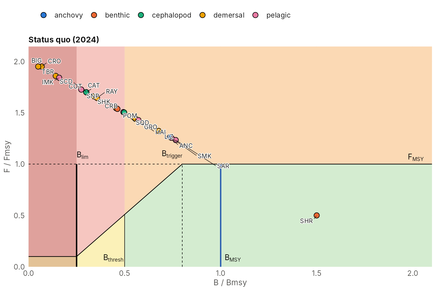
Every stock lies on the line B/Bmsy + F/Fmsy = 2 (the Schaefer equilibrium). Also check that every metier is fished (days by metier at the status quo):
x <- ms_simulate(sys, matrix(cap, 1), 200, capacity = matrix(cap, 1), gamma = 1.5, avg_years = 20)
round(colMeans(x$E_metier[, 1, ]))
#>  [1]  104 1659 1038  159   41  361   54   35   95  124
Part C: checklist for your own system
- Stocks. Collect r, K (or MSY and Bmsy), relative prices and, if relevant, seasonal availability; decide the F cap (persistence floor, default none; 1.95 keeps stocks at or above 0.05 Bmsy).
- Metiers. Define fishing tactics (gear, target) and grounds (depth zones, substrate, coastal zone); one row per tactic x ground.
-
Catchability. Either score an overlap matrix (main
fishery, by-catch, none) or describe habitats and grounds for
ms_landscape(). Only the shape of each stock’s column matters at this stage. - Segments. Home metiers and loyalty (zoning), efficiency (generalists below specialists), capacity (registered days) and the target share of days.
-
Behaviour. Choose
gamma(profit preference; 1.5 is a moderate default) and check where the days go. -
Calibrate.
ms_tune()for the day shares (with a status target), thenms_condition()if the status of each stock is known. - Check. Shares of days, B/Bmsy against the targets, every metier fished, the Kobe plot (stocks on the line B/Bmsy + F/Fmsy = 2), and the choke stock.
-
Save with
write_ms_system()and load withread_ms_system()or in the app (upload).
Next steps
-
Equilibrium analyses: yield curves
(
ms_yield_curve(),ms_shared_q_curve()) and the safeguarded MMSY (ms_optimise()); seevignette("mmsyFM"). -
Harvest strategies:
hcr_effort()with a minimum effort, phased changes, closures (all year or by month, e.g. 15 February to 15 May for the trawl grounds), assessed subsets, nominal assignment and complexes, under process, assessment and implementation error;ms_tune_hcr()to tune the triggers. -
The app:
run_app(), preset “Gulf of Thailand (draft)”, or upload the tables saved in step 3 of B4.